
[Apr 14, 2026] Genuine MO-210 Exam Dumps New 2026 Microsoft Pratice Exam
New 2026 Realistic MO-210 Dumps Test Engine Exam Questions in here
NEW QUESTION # 10
Instructions
Exam Environment
Exam Interface and Controls
The exam panel provides access to the project task(s). Each project has an associated file in which you will perform the project tasks.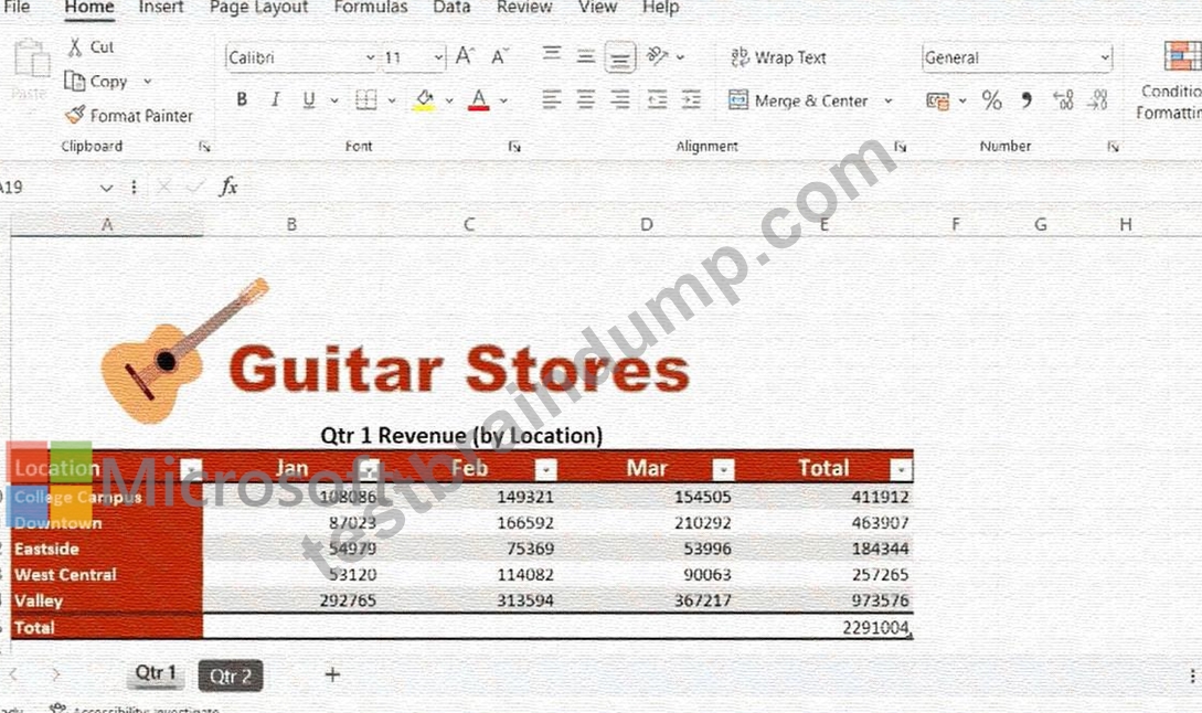
Overview:
Guitar Stores
You and a partner own several Guitar Stores. You are analyzing your revenue from the past two quarters.
Task 1:
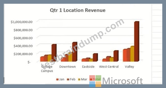
In the Qtr 1 worksheet change the configuration of the Q1 Location Revenue chart so that it displays the months on the x-axis and the revenue on they-axis.
Answer:
Explanation:
See the solution in Explanation below.
Explanation:
To swap the data on the axes so that the months appear on the x-axis and the revenue values appear on the y- axis, you will use theSwitch Row/Columnfeature in Excel.
Step 1: Select the Chart
* Go to theQtr 1worksheet.
* Click once on the border of theQ1 Location Revenuechart to select it. This will reveal theChart Design andFormattabs on the Ribbon.
Step 2: Switch Row/Column Data
* With the chart selected, click on theChart Designtab at the top of the window.
* Locate theDatagroup on the right side of the Ribbon.
* Click theSwitch Row/Columnbutton.
Step 3: Verify the Change
* The X-Axis (Horizontal):Should now display the month labels (Jan, Feb, Mar).
* The Legend:Should now display the differentLocations(College Campus, Downtown, etc.) as the colored series.
* The Y-Axis (Vertical):Will automatically scale to represent the revenue values.
NEW QUESTION # 11
Instructions
Exam Environment
Exam Interface and Controls
The exam panel provides access to the project task(s). Each project has an associated file in which you will perform the project tasks.
Overview:
Guitar Stores
You and a partner own several Guitar Stores. You are analyzing your revenue from the past two quarters.
Task 1:
On the Qtr 2 worksheet, in cell F10, insert a column sparkline showing the sales trend from Apr through Jun.
Apply Gold, Sparkline Style Accent 2,Darker 25% to the sparkline. Copy the sparkline to the remaining cells in the column, F11:F14.
Answer:
Explanation:
See the solution in Explanation below.
Explanation:
here is the step-by-step solution for Task 1:
Step 1: Navigate to the Correct Worksheet
Click on theQtr 2worksheet tab at the bottom of the Excel window to ensure you are working on the correct data set.
Step 2: Insert the Column Sparkline
* Click on cellF10(this is where the first sparkline will reside).
* Go to theInserttab on the Ribbon.
* In theSparklinesgroup, click onColumn.
* A dialog box will appear. ForData Range, select the cells representingApr through Junfor the first row (likelyB10:D10).
* Ensure theLocation Rangeis set to$F$10.
* ClickOK.
Step 3: Apply the Specific Sparkline Style
With cellF10still selected, a newSparklinetab will appear at the top of your Ribbon.
* Click on theSparklinetab.
* Click theMorearrow (the small downward arrow at the bottom right) of theStylesgallery to see all options.
* Hover over the styles to find the specific name:Gold, Sparkline Style Accent 2, Darker 25%.
* Click to apply it.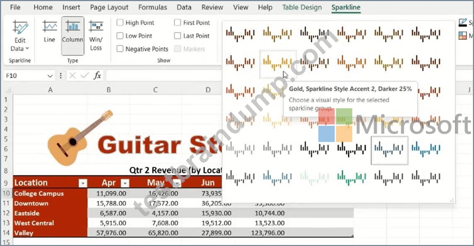
Step 4: Copy the Sparkline to Remaining Cells
* Select cellF10.
* Hover your mouse over theFill Handle(the small green square in the bottom-right corner of the cell).
* Click and drag the handle down to cellF14.
* Excel will automatically generate sparklines for the other locations (Downtown, Eastside, etc.) using the same style and corresponding data rows.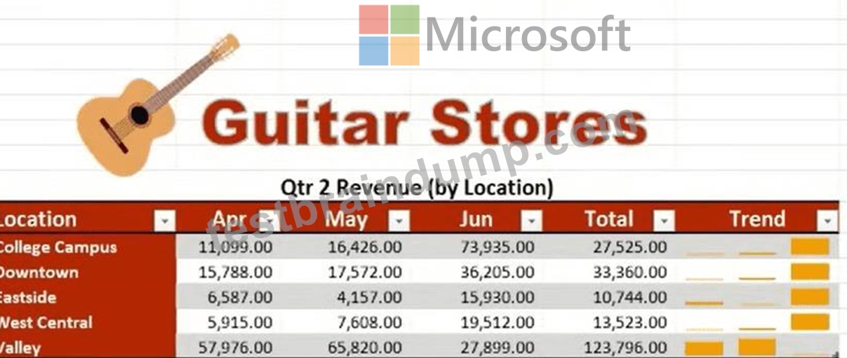
NEW QUESTION # 12
Instructions
Exam Environment
Exam Interface and Controls
The exam panel provides access to the project task(s). Each project has an associated file in which you will perform the project tasks.
Project 1
Overview:
Video Games
You are tracking video game popularity by compiling a workbook to document your findings.
Task 5:
Insert a Footer that displays today's date on the right and then return to Normal view.
Answer:
Explanation:
Here are the complete solutions below.
Explanation:
Project 1: Video Games - Task 5 Solution
Task:Insert a Footer that displays today's date on the right and then return to Normal view.
Step 1: Open the Header & Footer View
* Go to theInserttab on the Ribbon.
* Look for theTextgroup (usually near the right side).
* Click on theHeader & Footerbutton.
* Note:This will automatically switch your screen to "Page Layout" view, and you will see the header area at the top of the page.
Visual Reference:(Look for this icon in the Insert tab) [ Header & Footer ] Step 2: Navigate to the Footer
* You are currently in the Header. You need to go to theFooter.
* On theHeader & Footertab (which appears in the Ribbon when you are in this mode), click the button labeledGo to Footer.
* Alternative:You can simply scroll down to the bottom of the page until you see the footer boxes
"Click to add footer".
Visual Reference:(Button in the Navigation group) [ Go to Footer ]
Step 3: Select the Right Section
* The footer is divided into three boxes: Left, Center, and Right.
* Click inside theRightbox.
Visual Reference:[ Left Box ] [ Center Box ] [ *Click Here (Right Box)* ] Step 4: Insert the Current Date
* With your cursor flashing in the right footer box, look at theHeader & Footertab in the Ribbon.
* In theHeader & Footer Elementsgroup, click theCurrent Datebutton.
* You will see the code &[Date] appear in the box. This is correct; it will turn into the actual date once you click away.
Visual Reference:(Icon looks like a small calendar) [ Current Date ] -> Displays as &[Date] Step 5: Return to Normal View
* Clickanywhere inside the worksheet cells(outside the footer area) to apply the change.
* Go to theViewtab on the Ribbon.
* In theWorkbook Viewsgroup (far left), click onNormal.
Visual Reference:(View Tab > Workbook Views) [ Normal ]
Result:You have successfully added the date to the footer. In "Normal" view, you won't see the footer anymore, but it is there and will appear when printed.

NEW QUESTION # 13
Instructions
Exam Environment
Exam Interface and Controls
The exam panel provides access to the project task(s). Each project has an associated file in which you will perform the project tasks.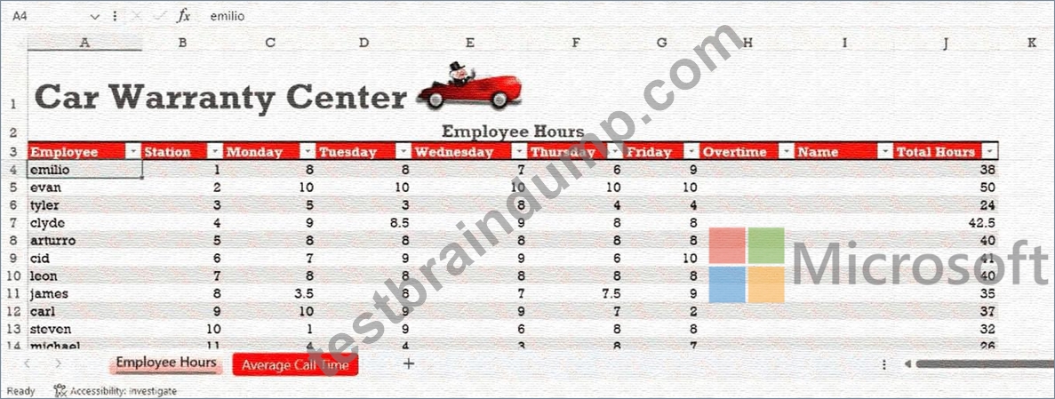
Overview:
Car Warranty
You are the supervisor for a Car Warranty Center. You use Excel to report employee hours and telephone calls.
Task 3:
Add a function to the Overtime column cell H4 on the Employee Hours worksheet that will display the word Yes if the value in cell J4 is higher than 40hours. otherwise display the word No. Copy the function from H4:
H16.
Answer:
Explanation:
See the solution in Explanation below.
Explanation:
To completeTask 3, you will use theIF functionto create a logical test that checks the total hours worked and returns a specific text result.
Step 1: Navigate to the Correct Cell
Ensure you are on theEmployee Hoursworksheet and click on cellH4(the first cell under theOvertime column).
Step 2: Enter the IF Function
Type the following formula into cellH4:
=IF(J4>40, "Yes", "No")
Breakdown of the formula:
* J4>40: This checks if the value in theTotal Hourscolumn is greater than 40.
* "Yes": The value to display if the condition isTrue.
* "No": The value to display if the condition isFalse.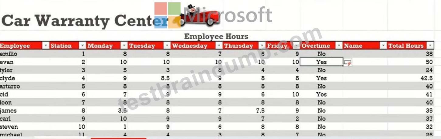
Step 3: Copy the Function (H4:H16)
Since your data is formatted as an Excel Table, the formula might automatically fill down. If it doesn't, follow these steps to copy it to the remaining cells:
* Click on cellH4to select it.
* Hover your mouse over thebottom-right cornerof the cell until the cursor turns into athin black cross (+).
* Click and dragthe handle down to cellH16.
* Release the mouse button to apply the logic to all employees.
Final Check
* Emilio (J4 = 38): Cell H4 should now displayNo.
* Evan (J5 = 50): Cell H5 should now displayYes.
NEW QUESTION # 14
Instructions
Exam Environment
Exam Interface and Controls
The exam panel provides access to the project task(s). Each project has an associated file in which you will perform the project tasks.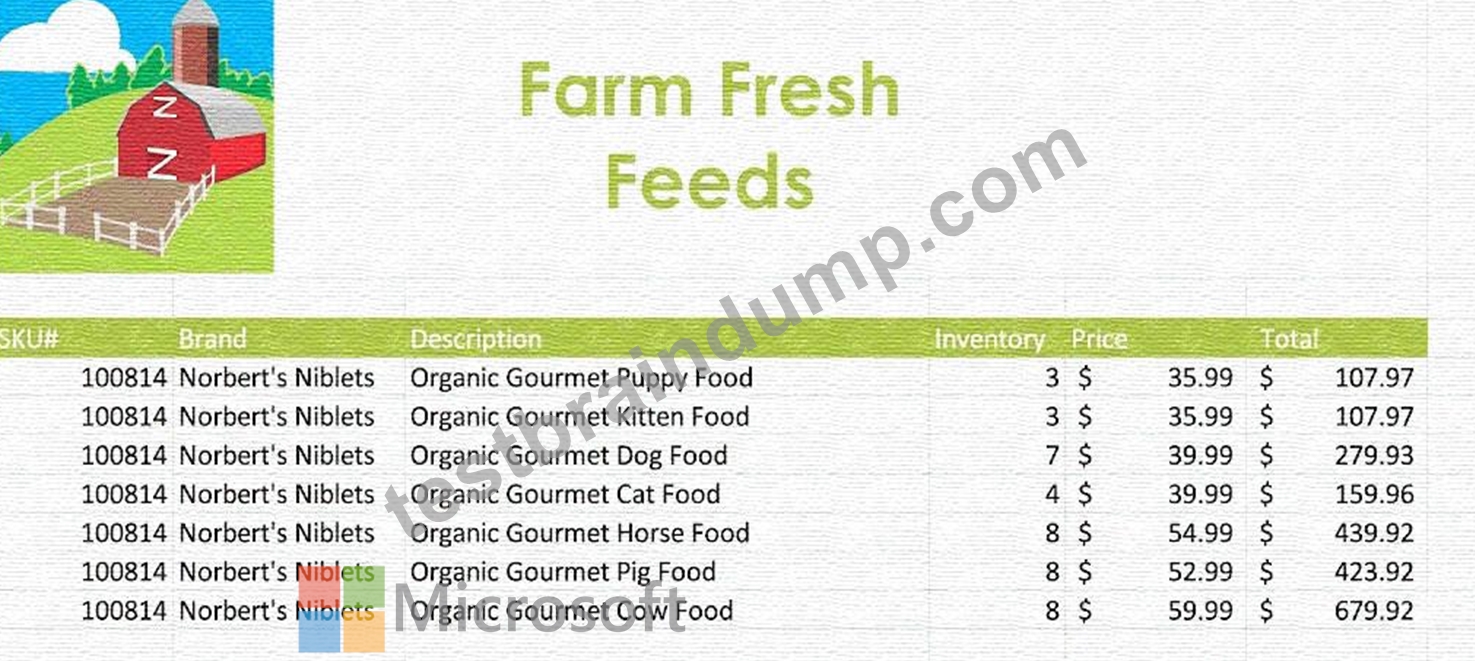
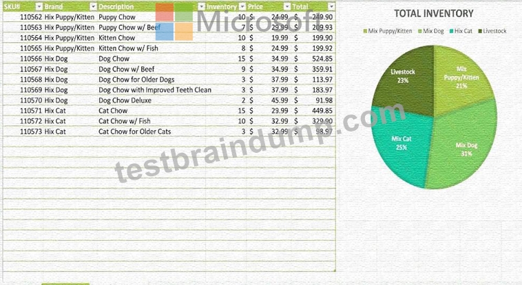
Farm Feeds:
You are the assistant manager for a farm pet feed store. You are creating an inventory report.
Task 1:
Remove the conditional formatting from the table on on the Feed Inventory worksheet.
Answer:
Explanation:
See the solution in Explanation below.
Explanation:
To completeTask 1: Remove the conditional formatting from the table on the Feed Inventory worksheet
, follow these steps:
Step 1: Select the Target Worksheet
First, ensure you are on the correct worksheet as specified in the instructions.
* Click on theFeed Inventorytab at the bottom of your Excel workbook.
Step 2: Select the Table or Data Range
You can remove formatting from the entire sheet, but to be precise with the "table," follow these sub-steps:
* Click anywhere inside the table (the area containing the SKU#, Brand, Description, etc.).
* PressCtrl + Ato select the entire table range.
Step 3: Access the Conditional Formatting Menu
* Go to theHometab on the top Ribbon.
* In theStylesgroup, click on theConditional Formattingbutton.
Step 4: Clear the Rules
* Hover your mouse overClear Rulesnear the bottom of the drop-down menu.
* A side menu will appear. SelectClear Rules from Selected Cells(if you have the table selected) or Clear Rules from Entire Sheetto ensure all formatting is removed.
Final Result
Once clicked, any data bars, color scales, or highlight rules (like the light green shading seen in your screenshot) that were applied via Conditional Formatting will be removed, leaving the standard table styling
NEW QUESTION # 15
Instructions
Exam Environment
Exam Interface and Controls
The exam panel provides access to the project task(s). Each project has an associated file in which you will perform the project tasks.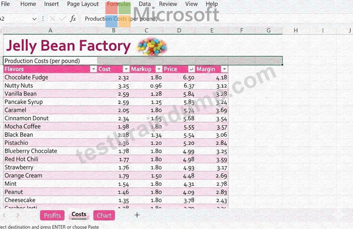

Overview:
Jelly Beans
A shop you manage sells gourmet jelly beans. You are tracking the amount of jelly beans sold each quarter and summarizing the information in aworkbook.
Task 4:
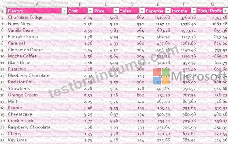
Filter the Profits worksheet to display only flavors with Total Profit that are Above Average.
Answer:
Explanation:
See the solution in Explanation below.
Explanation:
To filter theProfitsworksheet to display only the flavors with aTotal Profitthat isAbove Average, follow these steps:
Step 1: Access the Profits Worksheet
* Click on theProfitsworksheet tab at the bottom of the Excel window.
Step 2: Apply the Above Average Filter
* Look at theTotal Profitheader (CellG3). If you don't see a small drop-down arrow next to it, go to the Datatab and clickFilter.
* Click theFilter Drop-down Arrowin theTotal Profitheader cell.
* Hover your mouse overNumber Filtersin the menu that appears.
* From the side menu, selectAbove Average.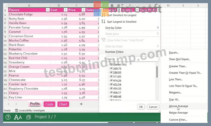
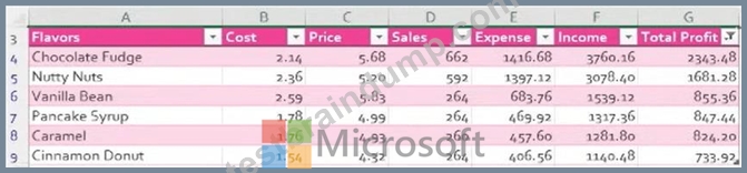
Step 3: Verify the Results
* Excel will automatically calculate the average of all values in the "Total Profit" column and hide any rows that fall below that number.
* You will notice the row numbers on the left are now blue, indicating a filter is active.
NEW QUESTION # 16
Instructions
Exam Environment
Exam Interface and Controls
The exam panel provides access to the project task(s). Each project has an associated file in which you will perform the project tasks.
Farm Feeds:
You are the assistant manager for a farm pet feed store. You are creating an inventory report.
Task 3:
On the Feed Inventory worksheet, remove the hyperlink functionality, but leave the text in cell C27.
Answer:
Explanation:
See the solution in Explanation below.
Explanation:
To completeTask 3: Remove the hyperlink functionality from cell C27 on the Feed Inventory worksheet, follow these specific steps to ensure the text remains while the link is deleted.
Step 1: Select the "Feed Inventory" Worksheet
Ensure you are on the correct sheet by clicking theFeed Inventorytab at the bottom of the window.
Step 2: Navigate to Cell C27
Locate cellC27in the Description column. Based on your project files, this is likely a URL or a linked piece of text at the bottom of the table.
Step 3: Remove the Hyperlink
You want to strip the "clickable" link without deleting the actual words inside the cell.
* Right-clickdirectly on cellC27.
* From the context menu that appears, selectRemove Hyperlink(it is usually located at the very bottom of the list).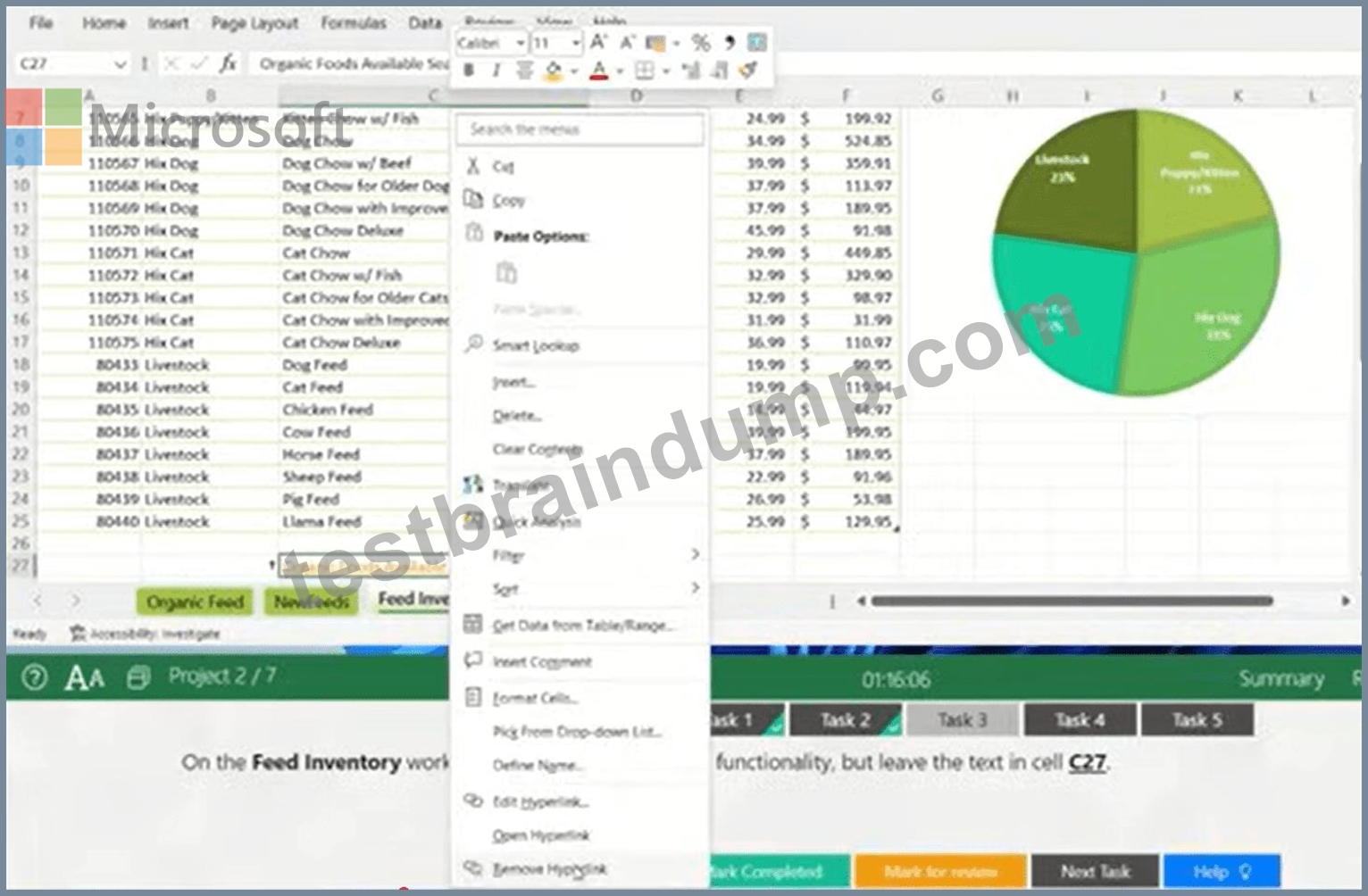
Step 4: Verify the Text Remains
The text should change from blue/underlined back to standard black text, but the characters themselves will stay in the cell.
NEW QUESTION # 17
Instructions
Exam Environment
Exam Interface and Controls
The exam panel provides access to the project task(s). Each project has an associated file in which you will perform the project tasks.
Project 1
Overview:
Video Games
You are tracking video game popularity by compiling a workbook to document your findings.
Task 4:
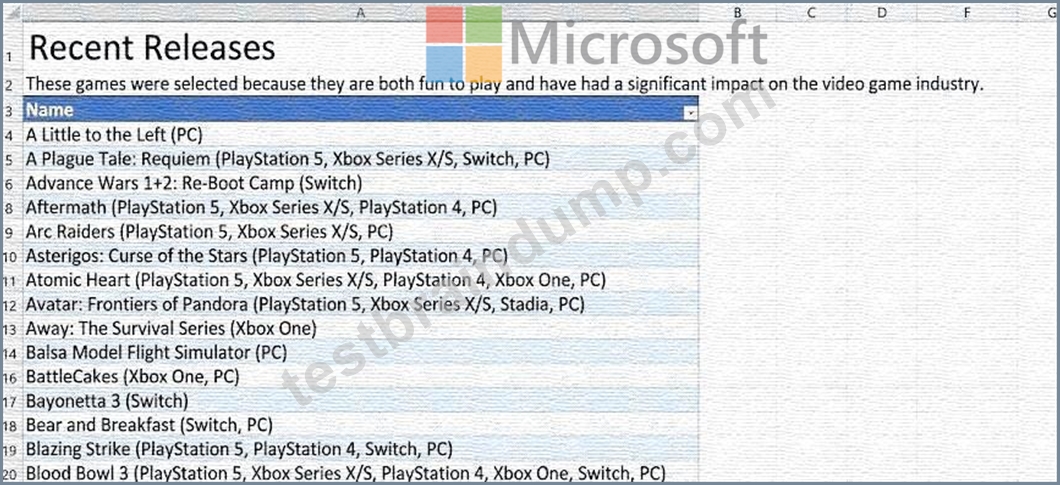
Convert the table on the Recent Releases worksheet to a cell range.
Answer:
Explanation:
Here are the complete solutions below.
Explanation:
Step 1: Select the Table
* Navigate to theRecent Releasesworksheet.
* Clickanywhereinside the data table (for example, click on the text "A Little to the Left").
* Note:You do not need to highlight the whole table; just clicking one cell inside it is enough to activate the hidden menu.
Step 2: Go to the "Table Design" Tab
* Look at the Ribbon at the very top of the Excel window.
* Because you clicked inside the table, a new tab calledTable Design(or sometimes justDesign) will appear on the far right side of the Ribbon.
* Click on theTable Designtab.
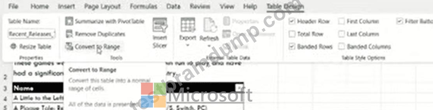
Step 3: Click "Convert to Range"
* In theTable Designtoolbar, look for theToolsgroup (usually on the left side).
* Click the button labeledConvert to Range.
Visual Reference:
Step 4: Confirm the Action
* A confirmation dialog box will pop up asking:"Do you want to convert the table to a normal range?"
* ClickYes.
Result:The table functionality (like the little filter arrows next to the headers) will disappear, but the cell colors and data will remain exactly where they are. The data is now a standard "Range."
NEW QUESTION # 18
Instructions
Exam Environment
Exam Interface and Controls
The exam panel provides access to the project task(s). Each project has an associated file in which you will perform the project tasks.
Overview:
Car Warranty
You are the supervisor for a Car Warranty Center. You use Excel to report employee hours and telephone calls.
Task 1:
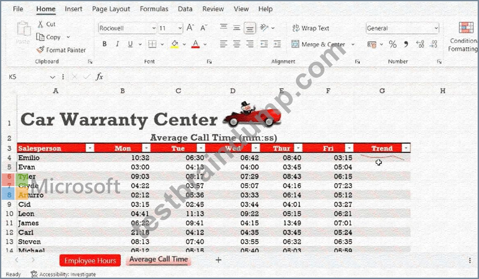
On the Average Call Time worksheet, use an Excel feature to copy the sparkline into all the vacant cells of the Trend column.
Answer:
Explanation:
See the solution in Explanation below.
Explanation:
n Excel 365, the most efficient way to do this is using theAutoFillfeature or simply dragging the fill handle.
Here is your step-by-step solution:
Step 1: Switch to the Correct Worksheet
Ensure you are on theAverage Call Timeworksheet. Click the red tab at the bottom of the screen to switch from the "Employee Hours" view (shown in your image) to the call time data.
Step 2: Identify the Sparkline
Locate the first cell in theTrendcolumn that already contains a Sparkline (likely cellF4or similar, depending on your layout).
Step 3: Use the Fill Handle to Copy
* Hover your mouse over thebottom-right cornerof the cell containing the sparkline.
* Your cursor will change from a thick white cross to athin black cross (+).
* Click and dragthe fill handle down to the bottom of the column to fill all the vacant cells in the
"Trend" column.
Pro Tip:Alternatively, you can simplydouble-clickthe thin black cross (fill handle), and Excel will automatically fill the sparklines down to the last row of your data.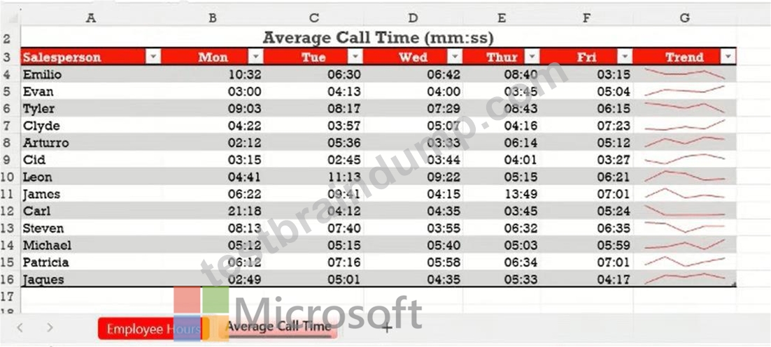
Alternative Method: Using the Ribbon
If you prefer using the menu interface:
* Select the cellwith the existing sparkline and all theempty cells below itwhere you want the sparklines to appear.
* Go to theHometab.
* In theEditinggroup, click theFillicon (downward arrow).
* SelectDown.
NEW QUESTION # 19
Instructions
Exam Environment
Exam Interface and Controls
The exam panel provides access to the project task(s). Each project has an associated file in which you will perform the project tasks.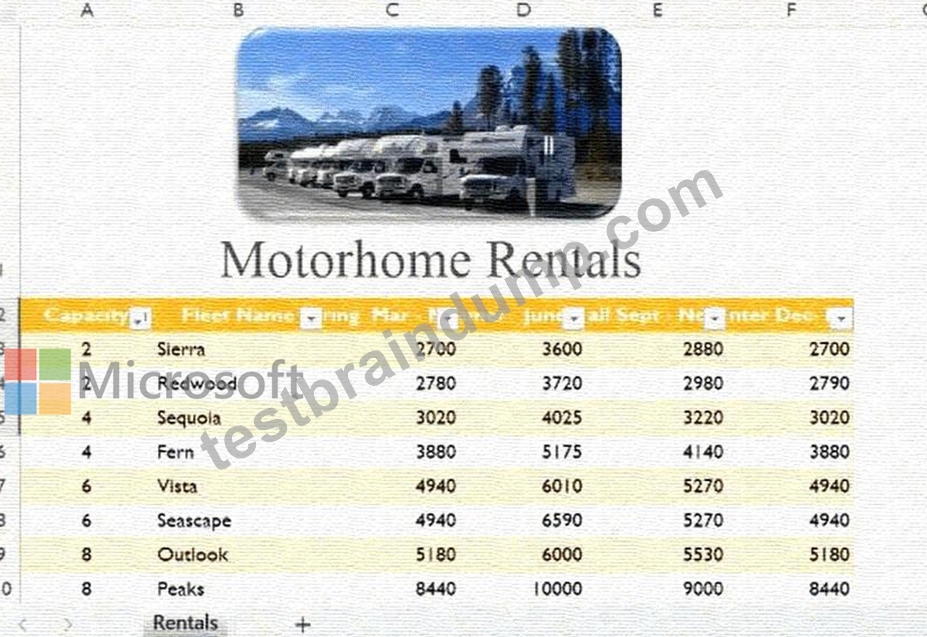
Overview:
Motorhome Rentals
Your company rents motorhomes. The motorhomes rent year-around at different prices. You are preparing pricing worksheets to be shared with others.
Task 2:
Add the value New Rates to the Title property of the document.
Answer:
Explanation:
See the solution in Explanation below.
Explanation:
To add a value to theTitleproperty of an Excel document, you need to access the Backstage view. This metadata is helpful for organizing and searching for files.
Step-by-Step Solution
* Click on theFiletab in the top-left corner of the Excel ribbon.
* Ensure thatInfois selected in the left-hand sidebar.
* On the right side of the screen, you will see a section labeledProperties.
* Locate the field namedTitle. If it says "Add a title," click directly on that text.
* TypeNew Ratesinto the text box.
* Click anywhere else on the screen or pressEnterto save the property.
* Click theBack arrowin the top-left corner to return to your worksheet.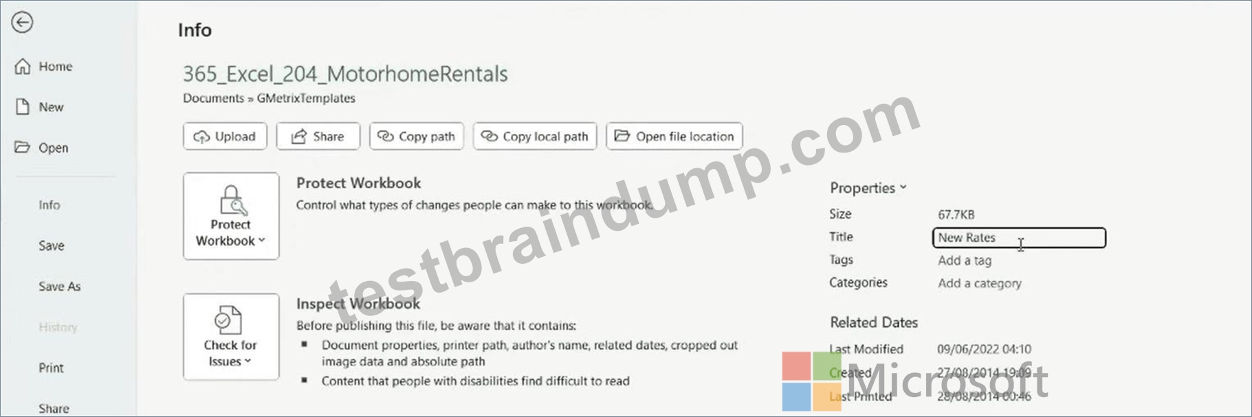
NEW QUESTION # 20
Instructions
Exam Environment
Exam Interface and Controls
The exam panel provides access to the project task(s). Each project has an associated file in which you will perform the project tasks.
Overview:
Jelly Beans
A shop you manage sells gourmet jelly beans. You are tracking the amount of jelly beans sold each quarter and summarizing the information in aworkbook.
Task 2:
Use a builtin Excel feature to copy all of the formatting of cell range A2:G2 located on the Profits worksheet and apply that formatting to cell A2 on theCosts worksheet.
Answer:
Explanation:
See the solution in Explanation below.
Explanation:
To transfer the formatting from theProfitsworksheet to theCostsworksheet while maintaining consistency, follow these steps:
Step 1: Copy the Source Formatting
* Click on theProfitsworksheet tab at the bottom of your Excel window.
* Select the cell rangeA2:G2.
* On theHometab, in theClipboardgroup, click theFormat Painterbutton (it looks like a paintbrush).
* Tip: Your cursor will now have a small paintbrush icon next to it, indicating the formatting is
"loaded" and ready to be pasted.
Step 2: Apply Formatting to the Destination
* Click on theCostsworksheet tab (the one shown in your provided image).
* Click directly onCell A2(the cell containing "Production Costs (per pound)").
* Excel will automatically apply the formatting across the range starting from A2 to match the original source.
Final Result
The cell range in theCostsworksheet should now match the style (font, background color, and borders) of the Profitsworksheet. The grey shading currently visible in your image in rangeB2:G2will be replaced by the style from the first sheet.
NEW QUESTION # 21
Instructions
Exam Environment
Exam Interface and Controls
The exam panel provides access to the project task(s). Each project has an associated file in which you will perform the project tasks.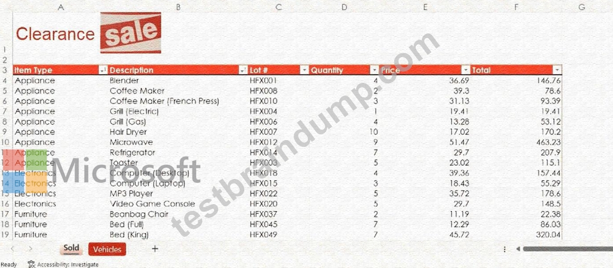
Overview:
Clearance Sale
You are the administrative assistant for a retail company that is going out of business. You've been tasked to prepare a workbook for the clearance sale.
Task 1:
On the Sold worksheet, insert a new column before column A.
Answer:
Explanation:
See the solution in Explanation below.
Explanation:
Task 1: Insert a new column before column A
To insert a new column at the very beginning of your worksheet, follow these steps:
* Select Column A: Click directly on the letter'A'at the top of the first column to select the entire column.
* Open the Insert Menu: There are two ways to do this:
* Option A (Right-Click): Right-click anywhere on the selected column and chooseInsertfrom the context menu.
* Option B (Ribbon): On theHometab, go to theCellsgroup, click the arrow next toInsert, and selectInsert Sheet Columns.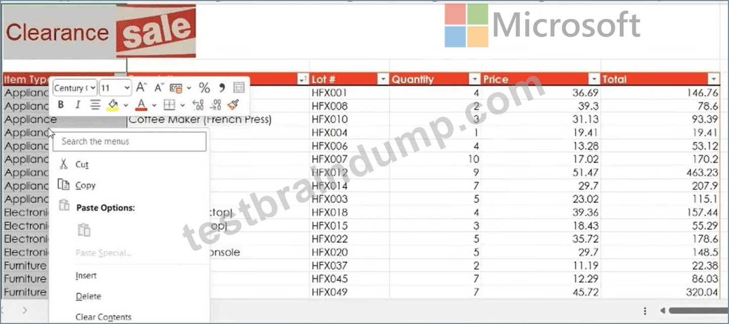
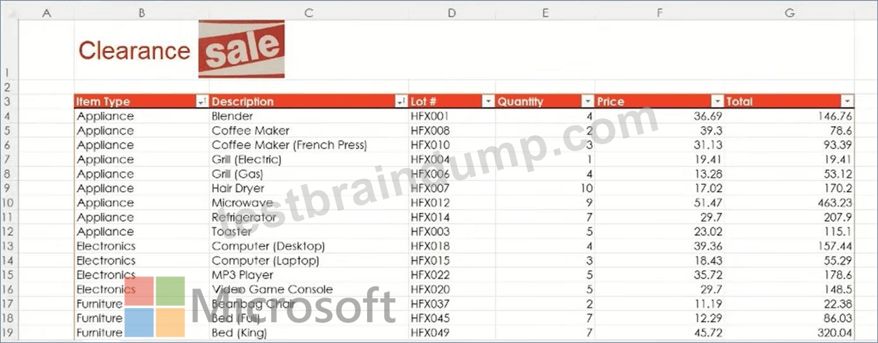
Verification
Once completed, your original "Item Type" column (previously Column A) will shift toColumn B, and you will have a brand new, emptyColumn Aat the start of your worksheet.
NEW QUESTION # 22
Instructions
Exam Environment
Exam Interface and Controls
The exam panel provides access to the project task(s). Each project has an associated file in which you will perform the project tasks.
Project 1
Overview:
Video Games
You are tracking video game popularity by compiling a workbook to document your findings.
Task 2:
On the Top 20 Videos worksheet, change the width of column C to 2.
Answer:
Explanation:
Here are the complete solutions below.
Explanation:
Step-by-Step Instructions
* Navigate to the Correct Worksheet:
* Click on the tab labeled Top 20 Videos at the bottom of the Excel window to ensure you are on the correct sheet.
* Select Column C:
* Click on the letter C in the column header to select the entire column.
* Open Column Width Settings:
* Method A (Ribbon): Go to the Home tab. In the Cells group (towards the right), click Format.
Select Column Width... from the dropdown menu.
* Method B (Right-click): Right-click directly on the column header "C". A context menu will appear. Click Column Width...
* Enter the Width:
* A small dialog box labeled "Column Width" will appear.
* Type 2 in the box.
* Click OK.
Visual Verification
Before: Column C (containing the "Year" data) is likely wider, fitting the four-digit years comfortably.
After: Column C will become very narrow. The "Year" header and the dates (like 2011, 1984) might display as hashes (####) because the column is now too narrow to display the numbers, or the text will simply be cut off. This is expected behavior for the exam task; do not widen it back out unless instructed to do so.
NEW QUESTION # 23
Instructions
Exam Environment
Exam Interface and Controls
The exam panel provides access to the project task(s). Each project has an associated file in which you will perform the project tasks.
Overview:
Car Warranty
You are the supervisor for a Car Warranty Center. You use Excel to report employee hours and telephone calls.
Task 2:
On the Employee Hours worksheet, add a row to the table that automatically calculates total hours worked by all employees.
Answer:
Explanation:
See the solution in Explanation below.
Explanation:
To completeTask 2, you need to enable theTotal Rowfeature for the table on theEmployee Hoursworksheet.
This is the most efficient way to automatically calculate sums in an Excel table.
Step 1: Select the Worksheet
Click on theEmployee Hourstab at the bottom of your Excel window to ensure you are on the correct sheet.
Step 2: Activate the Table
Click anywhere inside the data table (for example, click on cellA4where it says "emilio"). Once you click inside the table, a new tab calledTable Designwill appear at the very top of your Ribbon.
Step 3: Enable the Total Row
* Go to theTable Designtab on the Ribbon.
* In theTable Style Optionsgroup, check the box labeledTotal Row.
* Result:A new row labeled "Total" will immediately appear at the bottom of your data (Row 15).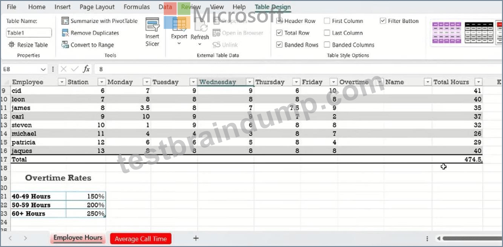
Step 4: Configure the Total Hours Calculation
By default, Excel might place a count or sum in the last column. You need to ensure theTotal Hourscolumn (Column J) is calculating correctly:
* Click on the cell at the bottom of theTotal Hourscolumn (J15).
* A smalldrop-down arrowwill appear next to the cell. Click it.
* SelectSumfrom the list.
Final Result
Your table will now have a dedicated row at the bottom that automatically updates the total hours whenever you add or change employee data.
NEW QUESTION # 24
......
Grab latest Amazon MO-210 Dumps as PDF Updated: https://www.testbraindump.com/MO-210-exam-prep.html
Updated Official licence for MO-210 Certified by MO-210 Dumps PDF: https://drive.google.com/open?id=1qmXfcK1xmnmNB86mGeHSz1ZE9YPCiBEz
